DIRAC on Human Glioblastoma — Vertical Tutorial¶

Goal: Run DIRAC on a real Human Glioblastoma spatial multi-omics sample (RNA + Protein/ADT), produce a joint embedding, cluster with Mclust, visualize spatial maps, and save all outputs (H5AD/CSV/PDF) for downstream analysis.

Table of Contents¶

Overview
Environment & Data
End-to-End Script (copy/paste)
Parameter Notes & Good Defaults
Outputs & File Saving
Reproducibility
Troubleshooting & Tips

1. Overview¶

Data: Human Glioblastoma with RNA and Protein (ADT) modalities.
Integration: DIRAC learns a joint embedding from RNA PCA + ADT expression using a spatial k-NN graph.
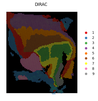
Clustering: mclust (via R) to obtain discrete domains (here n_clusters = 9).
Visualization: spatial clustering maps (PDF), colored by cluster assignments.
Artifacts: save AnnData objects, cluster CSV, and figures to a dedicated output folder.

2. Environment & Data¶

Dependencies (minimum)

Python ≥ 3.8
scanpy, anndata, numpy, matplotlib, pandas
R with package ``mclust`` (required for sd.utils.mclust_R)
DIRAC codebase locally available If not installed, follow: https://dirac-tutorial.readthedocs.io/en/latest/install.html

Paths used

data_path: ../DIRAC-main/data/Glioblastoma
data_name: Human_Glioblastoma
out_path: ./Results
save_path: ./Results/Human_Glioblastoma_DIRAC (auto-created)

Expected files

Human_Glioblastoma_RNA.h5ad
Human_Glioblastoma_Protein.h5ad

Download link:

3. End-to-End Script¶

At-a-glance map:

3.1–3.3 = prep & preprocessing
3.4 = build graph
3.5 = DIRAC training (joint embedding)
3.6 = write embedding
3.7 = clustering + spatial plot
3.8 = (Optional) Cross-omics mixing check — UMAP on the joint embedding
3.8 = save outputs (H5AD/CSV/PDF)

It uses GPU if available; otherwise set use_gpu=False.

3.1 Imports, fonts, paths, and seed¶

[1]:

import os
import pandas as pd
import numpy as np
import scanpy as sc
import matplotlib.pyplot as plt
import anndata
import matplotlib as mpl
mpl.rcParams['pdf.fonttype'] = 42
mpl.rcParams['ps.fonttype'] = 42

import sodirac as sd
sd.utils.seed_torch(seed=6)

data_path = "../DIRAC-main/data/Glioblastoma"
data_name = "Human_Glioblastoma"
methods = "DIRAC"
out_path = "./Results"
n_clusters = 9
save_path = os.path.join(out_path, f"{data_name}_{methods}")
if not os.path.exists(save_path):
    os.makedirs(save_path)

3.2 Load RNA/Protein and align cell order¶

[2]:

adata_RNA = sc.read(os.path.join(data_path,f"{data_name}_RNA.h5ad"))
adata_RNA.raw = adata_RNA
adata_RNA.var_names_make_unique()
adata_Protein = sc.read(os.path.join(data_path,f"{data_name}_Protein.h5ad"))
adata_Protein.raw = adata_Protein
adata_Protein = adata_Protein[adata_RNA.obs_names]

# adata_RNA = adata_RNA.copy()
adata_RNA.obsm["spatial"] = adata_RNA.obsm["spatial"].astype(float)
# adata_Protein = adata_Protein.copy()
adata_Protein.obsm["spatial"] = adata_Protein.obsm["spatial"].astype(float)

/home/project/11003054/changxu/Conda_envs/dirac-env/lib/python3.9/site-packages/anndata/_core/anndata.py:1820: UserWarning: Variable names are not unique. To make them unique, call `.var_names_make_unique`.
  utils.warn_names_duplicates("var")
/home/project/11003054/changxu/Conda_envs/dirac-env/lib/python3.9/site-packages/anndata/_core/anndata.py:1820: UserWarning: Variable names are not unique. To make them unique, call `.var_names_make_unique`.
  utils.warn_names_duplicates("var")
/tmp/ipykernel_3355960/3436773580.py:11: ImplicitModificationWarning: Setting element `.obsm['spatial']` of view, initializing view as actual.
  adata_Protein.obsm["spatial"] = adata_Protein.obsm["spatial"].astype(float)

3.3 Preprocess (RNA: filter/HVG/PCA; ADT: normalize/log/scale)¶

[3]:

######### Data processing
sc.pp.filter_genes(adata_RNA, min_cells=3)
sc.pp.normalize_total(adata_RNA)
sc.pp.log1p(adata_RNA)
sc.pp.highly_variable_genes(adata_RNA, n_top_genes=2000)
sc.pp.scale(adata_RNA)
sc.tl.pca(adata_RNA, n_comps=100)

sc.pp.normalize_total(adata_Protein)
sc.pp.log1p(adata_Protein)
sc.pp.scale(adata_Protein)

3.4 Build the spatial k-NN graph¶

[4]:

edge_index = sd.utils.get_single_edge_index(adata_RNA.obsm["spatial"], n_neighbors = 8)

Average neighbors per node (directed): 8.00 (edges=46048, nodes=5756)

3.5 Configure and train DIRAC¶

[5]:

dirac = sd.main.integrate_app(save_path = save_path, use_gpu = True, subgraph = False)
samples = dirac._get_data(dataset_list = [adata_RNA.obsm['X_pca'], adata_Protein.X], edge_index = edge_index)
models = dirac._get_model(samples, opt_GNN = "GAT")
data_z, combine_recon = dirac._train_dirac_integrate(samples = samples, models = models, scale_loss = 0.04, epochs = 300)

Found 2 unique domains.

DIRAC integrate..: 100%|█| 300/300 [0

3.6 Write back the joint embedding¶

[6]:

adata_RNA.obsm["DIRAC_embed"] = combine_recon
adata_Protein.obsm["DIRAC_embed"] = combine_recon

3.7 Cluster (MCLUST via R) and make a spatial plot¶

[7]:

# Optional: palette for up to ~30 clusters
colormaps = ["#E41A1C", "#377EB8", "#4DAF4A", "#984EA3", "#FF7F00", "#A65628", "#FFFF33", "#F781BF", "#999999",
        "#E5D8BD", "#B3CDE3", "#CCEBC5", "#FED9A6", "#FBB4AE", "#8DD3C7", "#BEBADA", "#80B1D3", "#B3DE69", "#FCCDE5",
        "#BC80BD", "#FFED6F", "#8DA0CB", "#E78AC3", "#E5C494", "#CCCCCC", "#FB9A99", "#E31A1C", "#CAB2D6", "#6A3D9A", "#B15928"]

sd.utils.mclust_R(adata=adata_RNA, num_cluster = n_clusters, used_obsm="DIRAC_embed",key_added="DIRAC")
sc.pl.spatial(adata_RNA, color=["DIRAC"], palette = colormaps, frameon=False, spot_size=200, show=False)
plt.savefig(os.path.join(save_path, f"{data_name}_{methods}_spatial.pdf"), bbox_inches='tight', dpi = 300)

R[write to console]:                    __           __
   ____ ___  _____/ /_  _______/ /_
  / __ `__ \/ ___/ / / / / ___/ __/
 / / / / / / /__/ / /_/ (__  ) /_
/_/ /_/ /_/\___/_/\__,_/____/\__/   version 6.0.0
Type 'citation("mclust")' for citing this R package in publications.

fitting ...
  |======================================================================| 100%

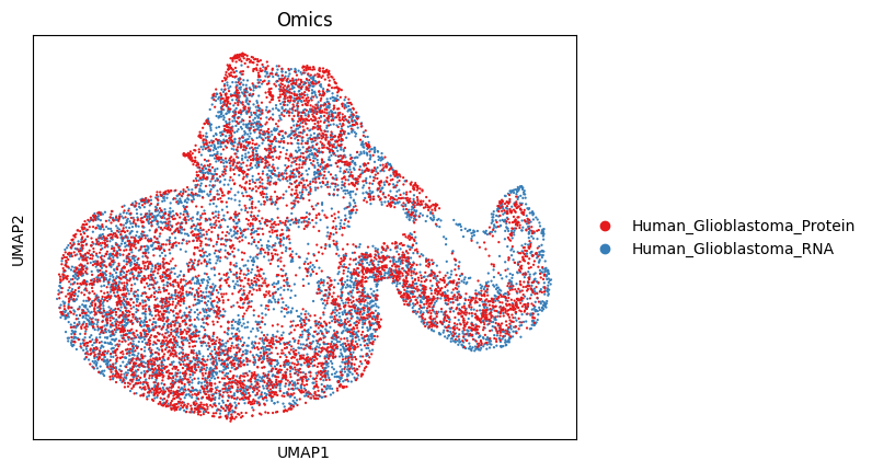
../_images/notebooks_run-Glioblastoma_18_2.png

3.8 (Optional) Cross-omics mixing check — UMAP on the joint embedding¶

What/why: After clustering the RNA layer, you may want to verify that RNA and Protein cells are well mixed in the shared embedding (i.e., integration worked). The snippet below:

tags each cell with its modality,
builds a combined AnnData from the joint embedding,
runs neighbors/UMAP + Leiden and MCLUST on the embedding,
plots UMAP colored by Omics, embed_mclust, and embed_leiden.

Assumption: data_z is the stacked embedding returned by DIRAC for all cells in the same order as dataset_list=[RNA, Protein], i.e. data_z = [RNA_rows; Protein_rows]. If your method returns a different ordering, reorder adata.obs accordingly before concatenation.

[8]:

# Label each modality for mixing diagnostics
adata_RNA.obs["Omics"] = data_name + "_RNA"
adata_RNA.obs["Omics"] = adata_RNA.obs["Omics"].astype("category")

adata_Protein.obs["Omics"] = data_name + "_Protein"
adata_Protein.obs["Omics"] = adata_Protein.obs["Omics"].astype("category")

# Build a combined AnnData on top of the joint embedding
# X := data_z so neighbors/UMAP use the learned space
adata = anndata.AnnData(data_z)
adata.obs = pd.concat([adata_RNA.obs, adata_Protein.obs], axis=0)

# Also store the embedding in obsm for methods that expect a named rep
adata.obsm[f"{methods}_embed"] = data_z

# UMAP over the joint space
sc.pp.neighbors(adata, use_rep="X")
sc.tl.umap(adata)

# Visualize modality mixing and clusters in UMAP
sc.pl.umap(adata, color="Omics", palette=colormaps, show=False)
plt.savefig(os.path.join(save_path, f"{data_name}_{methods}_embed_umap.pdf"), bbox_inches="tight", dpi=300)

../_images/notebooks_run-Glioblastoma_20_0.png

3.9 Save all artifacts (H5AD / CSV)¶

[9]:

adata_RNA.write(os.path.join(save_path, f"{data_name}_{methods}_RNA.h5ad"), compression="gzip")
adata_Protein.write(os.path.join(save_path, f"{data_name}_{methods}_Protein.h5ad"), compression="gzip")
adata_RNA.obs['DIRAC'].to_csv(os.path.join(save_path, f"{data_name}_{methods}.csv"))

4. Parameter Notes & Good Defaults¶

n_neighbors (graph): 6–12 are common. More neighbors → smoother neighborhoods; fewer → sharper boundaries.
RNA HVGs (``n_top_genes``): 2k–3k typical; trial 1–5k for sensitivity.
PCA components: 50–100 usually sufficient; large tissues can benefit from 100+.
GNN (``opt_GNN``): "GAT" (attentional, expressive), "SAGE" (efficient), "GCN" (simple).
n_hiddens / n_outputs: start at 128 / 64; increase for complex tissues, reduce for memory.
epochs: 200–400 typical for stable embeddings.
lamb (regularization): ↑ if overfitting; ↓ if underfitting.
scale_loss: balances reconstruction and other terms; small tweaks (0.02–0.06) can help.
n_clusters (MCLUST): use prior knowledge or grid-search; Leiden is an alternative if R/mclust is unavailable.
spot_size: adapt to the platform’s spot diameter for best visual density.

Optional subgraph mode

For very large samples or limited VRAM: initialize integrate_app(..., subgraph=True) and pass num_parts in _get_data(...) to split the graph.
Larger num_parts → lower peak memory but more overhead.

5. Outputs & File Saving¶

Figures: Results/Human_Glioblastoma_DIRAC/Human_Glioblastoma_DIRAC_Combined_spatial.pdf
AnnData: Results/Human_Glioblastoma_DIRAC/Human_Glioblastoma_DIRAC_RNA.h5ad Results/Human_Glioblastoma_DIRAC/Human_Glioblastoma_DIRAC_Protein.h5ad
Labels (CSV): Results/Human_Glioblastoma_DIRAC/Human_Glioblastoma_DIRAC.csv (column = DIRAC)

What’s inside

obsm["DIRAC_embed"]: shared embedding for downstream neighbors/UMAP.
obs["DIRAC"]: MCLUST cluster labels (strings).
uns often contains plotting metadata after scanpy calls.

6. Reproducibility¶

Set deterministic seeds: sd.utils.seed_torch(seed=6) (already in the script).
Minor non-determinism may persist on GPU due to cuDNN; results should be qualitatively stable.

Ready to go: Copy the End-to-End Script into your notebook, adjust paths if needed, and run. The tutorial above explains each choice so users can reproduce and extend your results confidently.