DIRAC Spatial Multi-Omics — Vertical Integration
Goal: Integrate spatial RNA, Protein (ADT), and ATAC with DIRAC, then cluster and visualize tissue structure. This guide walks through data loading, preprocessing, graph construction, integration, clustering, visualization, and evaluation.
Table of Contents
Environment & Data
Load Packages
Load Modalities
Preprocess
Build the Spatial Graph
Two-Omics Integration (RNA + ADT)
Clustering & Evaluate (ARI) & Visualization
Auto-select resolution by maximizing the Calinski–Harabasz score
Extend to Three Omics (add ATAC)
Subgraph Training (Optional)
Tips & Troubleshooting
1. Environment & Data
Dependencies
Python ≥ 3.8
scanpy,anndata,numpy,matplotlib,scikit-learnDIRAC codebase locally available (added to
sys.path). If not installed, follow the official guide: Install DIRAC
Download NSF Data
Source (three modalities):
RNA (gene expression)
ADT / Protein
ATAC (chromatin accessibility)
Download link:
2. Load Packages
[1]:
import os
import scanpy as sc
import numpy as np
import sys
import matplotlib.pyplot as plt
import anndata
from sklearn.metrics.cluster import adjusted_rand_score

import sodirac as sd
sd.utils.seed_torch(seed=0)

data_path = "../DIRAC-main/data/NSF"
save_path = './Results'
methods = "DIRAC"
n_clusters = 5
3. Load Modalities
Read the AnnData objects for RNA and ADT (and later ATAC).
Assumptions
adata.obsm[“spatial”] contains spatial coordinates.
adata.obs[“ground_truth”] provides labels for evaluation (simulated dataset).
[2]:
adata_RNA = anndata.read_h5ad(os.path.join(data_path, "sim_RNA.h5ad"))
adata_Protein = anndata.read_h5ad(os.path.join(data_path, "sim_ADT.h5ad"))
print(adata_RNA);print(adata_Protein)
AnnData object with n_obs × n_vars = 4096 × 2000
    obs: 'ground_truth'
    obsm: 'spatial'
AnnData object with n_obs × n_vars = 4096 × 100
    obs: 'ground_truth'
    obsm: 'spatial'
4. Preprocess
(Standard normalization/log-transform/scale for RNA & ADT; PCA for RNA.)
Why these steps?
Makes modalities comparable and denoised before graph-based integration.
PCA yields a compact representation for RNA to feed into the GNN.
[3]:
sc.pp.filter_genes(adata_RNA, min_cells=3)
sc.pp.normalize_total(adata_RNA)
sc.pp.log1p(adata_RNA)
sc.pp.scale(adata_RNA)
sc.tl.pca(adata_RNA, n_comps=50)

sc.pp.normalize_total(adata_Protein)
sc.pp.log1p(adata_Protein)
sc.pp.scale(adata_Protein)
5. Build the Spatial Graph
(Construct a graph over spatial coordinates. Start with k-NN; use radius when platform resolution requires explicit distance control.)
# Option A: k-NN (recommended starting point)
edge_index = sd.utils.get_single_edge_index(
    adata_RNA.obsm["spatial"],
    n_neighbors=8,
    graph_methods="knn"
)

# Option B: radius (tune n_radius to match platform resolution)
edge_index = sd.utils.get_single_edge_index(
    adata_RNA.obsm["spatial"],
    n_radius=0.1,
    graph_methods="radius"
)
Note
Different spatial platforms have different spot sizes/resolutions; for radius graphs, tune n_radius until neighborhoods look reasonable.
[4]:
edge_index = sd.utils.get_single_edge_index(adata_RNA.obsm["spatial"], n_neighbors = 8, graph_methods='knn')
Average neighbors per node (directed): 8.00 (edges=32768, nodes=4096)
6. Two-Omics Integration (RNA + ADT)
[5]:
dirac = sd.main.integrate_app(save_path = save_path, use_gpu = True, subgraph = False)
samples = dirac._get_data(dataset_list = [adata_RNA.obsm['X_pca'], adata_Protein.X], edge_index = edge_index)
models = dirac._get_model(samples)
data_z, combine_recon = dirac._train_dirac_integrate(samples = samples, models = models, epochs = 200)
adata_RNA.obsm["DIRAC_embed"] = combine_recon
adata_Protein.obsm["DIRAC_embed"] = combine_recon
Found 2 unique domains.
DIRAC integrate..: 100%|█| 200/200 [0
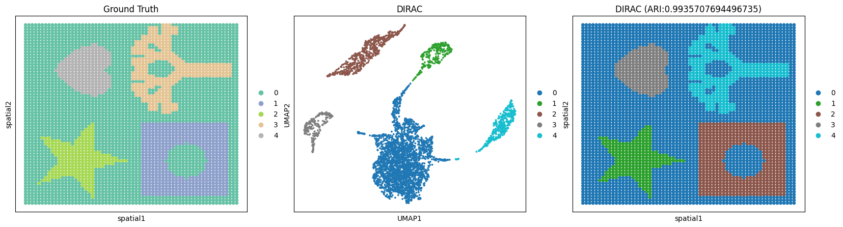
7. Clustering & Compute ARI & Visualization
(Use Leiden or MCLUST; below shows mclust in 9))
# Option B: Mclust (requires R + mclust)
sd.utils.mclust_R(adata_RNA, num_cluster=n_clusters)
Interpretation
ARI ≈ 1.0 → perfect match
ARI ≈ 0 → random alignment
ARI < 0 → worse than random
[6]:
sc.pp.neighbors(adata_RNA, use_rep="DIRAC_embed", n_neighbors=15)
res = sd.utils._priori_cluster(adata_RNA, eval_cluster_n = n_clusters)
sc.tl.leiden(adata_RNA, resolution = res, key_added="DIRAC", flavor="igraph", n_iterations=2, directed=False)
sc.tl.umap(adata_RNA)
ARI = float(adjusted_rand_score(adata_RNA.obs['DIRAC'], adata_RNA.obs['ground_truth']))

fig, ax_list = plt.subplots(1, 3, figsize=(20, 5))
sc.pl.embedding(adata_RNA, basis='spatial', color='ground_truth', title='Ground Truth', s=100, show=False, palette="Set2", ax=ax_list[0])
sc.pl.umap(adata_RNA, color='DIRAC', title='DIRAC', s=30, show=False, palette="tab10", ax=ax_list[1])
sc.pl.embedding(adata_RNA, basis='spatial', color='DIRAC', title=f'DIRAC (ARI:{ARI})', s=100, show=False, palette="tab10", ax=ax_list[2])
Best resolution: 0.02
[6]:
<Axes: title={'center': 'DIRAC (ARI:0.9935707694496735)'}, xlabel='spatial1', ylabel='spatial2'>
8. Auto-select resolution by maximizing the Calinski–Harabasz score
How it works:
Prior-free: Users do not provide n_clusters; only the data are required.
Resolution sweep: Run Leiden across a grid of resolutions (e.g., 0.01–2.5, step 0.01).
Internal validity: For each partition, compute the Calinski–Harabasz score, which balances within-cluster compactness and between-cluster separation.
Model selection: Pick the resolution with the highest CH score; this implicitly fixes the number of spatial niches (clusters).
[7]:
res = sd.utils._optimize_cluster(adata_RNA)
sc.tl.leiden(adata_RNA, resolution = res, key_added="DIRAC", flavor="igraph", n_iterations=2, directed=False)
sc.tl.umap(adata_RNA)
ARI = float(adjusted_rand_score(adata_RNA.obs['DIRAC'], adata_RNA.obs['ground_truth']))

fig, ax_list = plt.subplots(1, 3, figsize=(20, 5))
sc.pl.embedding(adata_RNA, basis='spatial', color='ground_truth', title='Ground Truth', s=100, show=False, palette="Set2", ax=ax_list[0])
sc.pl.umap(adata_RNA, color='DIRAC', title='DIRAC', s=30, show=False, palette="tab10", ax=ax_list[1])
sc.pl.embedding(adata_RNA, basis='spatial', color='DIRAC', title=f'DIRAC (ARI:{ARI})', s=100, show=False, palette="tab10", ax=ax_list[2])
Best resolution: 0.01
[7]:
<Axes: title={'center': 'DIRAC (ARI:0.9935707694496735)'}, xlabel='spatial1', ylabel='spatial2'>

9. Extend to Three Omics (add ATAC)
[8]:
adata_ATAC = anndata.read_h5ad(os.path.join(data_path, "sim_ATAC.h5ad"))
print(adata_ATAC)

sc.pp.filter_genes(adata_ATAC, min_cells=3)
sd.utils.lsi(adata_ATAC, n_comps=100)

dirac = sd.main.integrate_app(save_path = save_path, use_gpu = True, subgraph = False)
samples = dirac._get_data(dataset_list = [adata_RNA.obsm['X_pca'], adata_Protein.X, adata_ATAC.obsm['X_lsi']], edge_index = edge_index)
models = dirac._get_model(samples,opt_GNN = "GAT")
data_z, combine_recon  = dirac._train_dirac_integrate(samples = samples,models = models,epochs = 200)

adata_RNA.obsm["DIRAC_embed"] = combine_recon
sc.pp.neighbors(adata_RNA, use_rep="DIRAC_embed")
sd.utils.mclust_R(adata_RNA, num_cluster=n_clusters, used_obsm="DIRAC_embed", key_added="DIRAC")
sc.tl.umap(adata_RNA)
ARI = float(adjusted_rand_score(adata_RNA.obs['DIRAC'], adata_RNA.obs['ground_truth']))

fig, ax_list = plt.subplots(1, 3, figsize=(20, 5))
sc.pl.embedding(adata_RNA, basis='spatial', color='ground_truth', title='Ground Truth', s=100, show=False, palette="Set2", ax=ax_list[0])
sc.pl.umap(adata_RNA, color='DIRAC', title='DIRAC', s=30, show=False, palette="tab10", ax=ax_list[1])
sc.pl.embedding(adata_RNA, basis='spatial', color='DIRAC', title=f'DIRAC (ARI:{ARI})', s=100, show=False, palette="tab10", ax=ax_list[2])
AnnData object with n_obs × n_vars = 4096 × 4000
    obs: 'ground_truth'
    obsm: 'spatial'
Found 3 unique domains.
DIRAC integrate..: 100%|█| 200/200 [0
R[write to console]:                    __           __
   ____ ___  _____/ /_  _______/ /_
  / __ `__ \/ ___/ / / / / ___/ __/
 / / / / / / /__/ / /_/ (__  ) /_
/_/ /_/ /_/\___/_/\__,_/____/\__/   version 6.0.0
Type 'citation("mclust")' for citing this R package in publications.
fitting ...
  |======================================================================| 100%
[8]:
<Axes: title={'center': 'DIRAC (ARI:0.994213907242581)'}, xlabel='spatial1', ylabel='spatial2'>

10. Subgraph Training (Optional)
(Enable subgraph=True for large tissues or memory constraints.)
Key idea: turn on subgraph mode at app creation, and set
num_partsin_get_datato control how many subgraphs you split into.
When to use
Very large graphs
Limited GPU RAM
[9]:
dirac = sd.main.integrate_app(save_path = save_path, use_gpu = True, subgraph = True)
samples = dirac._get_data(dataset_list = [adata_RNA.obsm['X_pca'], adata_Protein.X, adata_ATAC.obsm['X_lsi']],\
                          edge_index = edge_index, num_parts = 5)
models = dirac._get_model(samples, opt_GNN = "GAT")
data_z, combine_recon  = dirac._train_dirac_integrate(samples = samples, models = models, epochs = 200)

adata_RNA.obsm["DIRAC_embed"] = combine_recon
sc.pp.neighbors(adata_RNA, use_rep="DIRAC_embed")
sd.utils.mclust_R(adata_RNA, num_cluster=n_clusters, used_obsm="DIRAC_embed", key_added="DIRAC")
sc.tl.umap(adata_RNA)
ARI = float(adjusted_rand_score(adata_RNA.obs['DIRAC'], adata_RNA.obs['ground_truth']))

fig, ax_list = plt.subplots(1, 3, figsize=(20, 5))
sc.pl.embedding(adata_RNA, basis='spatial', color='ground_truth', title='Ground Truth', s=100, show=False, palette="Set2", ax=ax_list[0])
sc.pl.umap(adata_RNA, color='DIRAC', title='DIRAC', s=30, show=False, palette="tab10", ax=ax_list[1])
sc.pl.embedding(adata_RNA, basis='spatial', color='DIRAC', title=f'DIRAC (ARI:{ARI})', s=100, show=False, palette="tab10", ax=ax_list[2])
Computing METIS partitioning...
Done!
Found 3 unique domains.
DIRAC integrate..: 100%|█| 200/200 [0
fitting ...
  |======================================================================| 100%
[9]:
<Axes: title={'center': 'DIRAC (ARI:0.9957281504554227)'}, xlabel='spatial1', ylabel='spatial2'>

11. Tips & Troubleshooting
DIRAC install: If DIRAC is not installed, follow → https://dirac-tutorial.readthedocs.io/en/latest/install.html
GPU vs CPU: Set use_gpu=True if CUDA is available; otherwise False (training will be slower).
Graph choice: Start with k-NN; consider radius when platform spot sizes demand explicit distance thresholds (tune n_radius).
Mclust: Requires R with mclust on PATH; if not available, use Leiden.
Scaling & LSI: Keep RNA/ADT standardized; use LSI for ATAC.
Reproducibility: Seeds help, but GPU nondeterminism (cuDNN) may still cause minor drifts.
Memory: Reduce n_hiddens/n_outputs, enable subgraph=True, or decrease neighborhood sizes if you hit OOM.