DIRAC Spatial Multi-Omics — Horizontal Integration¶

Horizontal annotation with DIRAC. This Quickstart explains how the demo runs and what each step does, for both single-modality (RNA→RNA) and dual-modality (RNA+ATAC→RNA+ATAC) annotation using spatial graphs, plus an optional novel cell type discovery stage.

Table of Contents¶

Overview & Scope
Environment & Data
Load Packages
Single-Modality Annotation (RNA → RNA)
Metrics & Visualization
Dual-Modality Annotation (RNA+ATAC → RNA+ATAC)
Novel Cell Type Discovery (Confidence Filtering)
Tips & Troubleshooting

1. Overview & Scope¶

Goal: Transfer cell type labels from a source dataset to a target dataset (horizontal integration) using DIRAC with spatial graphs.
Included in this demo:
1. Single-modality annotation: RNA → RNA
2. Dual-modality annotation: RNA+ATAC → RNA+ATAC (feature concatenation with explicit modality splits)
3. Optional novel-cell discovery: apply confidence filtering (e.g., threshold = 0.9) so low-confidence predictions are marked “unassigned”, revealing putative missing/unknown cell types when the reference is incomplete.

High-level flow

Load AnnData for source and target.
Preprocess each dataset (normalize → log1p → scale).
Build spatial graphs: multi-batch (source) and single-sample (target).
Initialize DIRAC’s annotate_app.
Package data via _get_data(...) (optionally split into subgraphs with num_parts_*).
Build a GNN via _get_model(...) (e.g., GraphSAGE or GAT).
Train _train_dirac_annotate(...) to learn features & predict labels on the target.
(Optional) Enable confidence filtering during training to tag low-confidence predictions as "unassigned"; tune confidence_threshold (e.g., 0.8–0.95) based on data quality and reference completeness.
Write back embeddings/predictions; evaluate accuracy/precision/recall/F1 on assigned cells, report Unassigned Rate, and visualize spatial maps and confidence.

2. Environment & Data¶

Dependencies

Python ≥ 3.9
scanpy, anndata, numpy, matplotlib, scikit-learn, torch
DIRAC codebase available. If not installed, follow: https://dirac-tutorial.readthedocs.io/en/latest/install.html

Paths used in the demo

data_path: ../DIRAC-main/data/scMultiSim
save_path: ./Results
methods tag: "DIRAC"

Expected input files

Single-modality: source_RNA.h5ad, target_RNA.h5ad
Dual-modality: additionally source_ATAC.h5ad, target_ATAC.h5ad

Required fields in the AnnData

obsm["spatial"] for spatial coordinates (source & target)
obs["batch"] for source (used by multi-batch graph building)
obs["cell.type"] for source labels and target ground truth (for metrics)

Download link:

We use scMultiSim benchmark data with mask = 0.3.

https://drive.google.com/drive/folders/1GK_Ij0bVL9tRoHbBrYAjeywCB4ux5S-D?usp=drive_link

What “mask = 0.3” means (important)

A dropout mask is applied independently to both RNA and ATAC matrices.
Roughly 30% of entries are randomly set to zero (element-wise), i.e., random sparsification at rate 0.3 in each modality.

3. Load Packages¶

[1]:

import os
import scanpy as sc
import numpy as np
import matplotlib.pyplot as plt
import anndata
import sklearn

import sodirac as sd
sd.utils.seed_torch(seed=0)

data_path = "../DIRAC-main/data/scMultiSim"
save_path = './Results'
methods = "DIRAC"

4. Single-Modality Annotation (RNA → RNA)¶

What this part does

Uses RNA only. Learns from source_RNA.h5ad (with cell types) and predicts labels for target_RNA.h5ad.
Builds a multi-batch spatial graph for source (accounts for obs["batch"]) and a single-sample spatial graph for target.

Step-by-step (as in your script)

[2]:

# 1) Load source/target
source_RNA = anndata.read_h5ad(os.path.join(data_path, "source_RNA.h5ad"))
target_RNA = anndata.read_h5ad(os.path.join(data_path, "target_RNA.h5ad"))
print(source_RNA); print(target_RNA)

# 2) Preprocess (normalize → log1p → scale)
sc.pp.normalize_total(source_RNA)
sc.pp.log1p(source_RNA)
sc.pp.scale(source_RNA)

sc.pp.normalize_total(target_RNA)
sc.pp.log1p(target_RNA)
sc.pp.scale(target_RNA)

# 3) Spatial graphs
#  - Source: multi-batch kNN graph (uses spatial + batch)
source_edge_index = sd.utils.get_multi_edge_index(source_RNA.obsm["spatial"], source_RNA.obs["batch"], n_neighbors=10)
#  - Target: single-sample kNN graph
target_edge_index = sd.utils.get_single_edge_index(target_RNA.obsm["spatial"], n_neighbors=10)

# 4) Initialize DIRAC annotation app
annotate = sd.main.annotate_app(save_path=save_path, use_gpu=True)

# 5) Package data for training
samples = annotate._get_data(
        source_data=source_RNA.X,
        source_label=source_RNA.obs["cell.type"],
        source_edge_index=source_edge_index,
        target_data=target_RNA.X,
        target_edge_index=target_edge_index,
        num_parts_source=source_RNA.shape[0] // 200,
        num_parts_target=target_RNA.shape[0] // 200,
    )

# 6) Build model (GraphSAGE in this demo)
models = annotate._get_model(samples=samples)

# 7) Train
results = annotate._train_dirac_annotate(samples=samples, models=models, n_epochs=100)
# np.savez(os.path.join(save_path, "DIRAC_results.npz"), **results)

# 8) Write back embeddings & predictions
source_RNA.obsm[f"{methods}_embed"] = results["source_feat"]
target_RNA.obsm[f"{methods}_embed"] = results["target_feat"]
target_RNA.obs[f"{methods}_pred"] = results["target_pred"]
target_RNA.obs[f"{methods}"] = target_RNA.obs[f"{methods}_pred"].map(results["pairs"])

AnnData object with n_obs × n_vars = 11971 × 200
    obs: 'pop', 'depth', 'cell.type', 'cell.type.idx', 'batch'
    obsm: 'spatial'
AnnData object with n_obs × n_vars = 3029 × 200
    obs: 'pop', 'depth', 'cell.type', 'cell.type.idx', 'batch'
    obsm: 'spatial'
Average neighbors per node (directed): 10.00 (edges=119710, nodes=11971)
Average neighbors per node (directed): 10.00 (edges=30290, nodes=3029)
Identified 2 unique domains.

Computing METIS partitioning...
Done!
Computing METIS partitioning...
Done!
DIRAC annotate training..: 100%|█| 10

5. Metrics & Visualization¶

Metrics (weighted, as in your script)

Accuracy, Precision (weighted), Recall (weighted), F1 (weighted) using sklearn.

Spatial visualization

Compare ground truth vs predicted labels on the target:

[3]:

metrics_all = {
            "Accuracy Score":
                float(sklearn.metrics.accuracy_score(target_RNA.obs["cell.type"], target_RNA.obs[f"{methods}"])),
            "Precision Score":
                float(sklearn.metrics.precision_score(target_RNA.obs["cell.type"], target_RNA.obs[f"{methods}"], average='weighted')),
            "Recall Score":
                float(sklearn.metrics.recall_score(target_RNA.obs["cell.type"], target_RNA.obs[f"{methods}"], average='weighted')),
            "F1 Score":
                float(sklearn.metrics.f1_score(target_RNA.obs["cell.type"], target_RNA.obs[f"{methods}"], average='weighted'))}
print(metrics_all)

sc.pl.embedding(target_RNA, basis='spatial', color=['cell.type', f'{methods}'], title=['Ground truth',f"{methods} ACC {metrics_all['Accuracy Score']}"], s=50, show=False)

{'Accuracy Score': 0.880488610102344, 'Precision Score': 0.8821684104621875, 'Recall Score': 0.880488610102344, 'F1 Score': 0.8804397263487906}

[3]:

[<Axes: title={'center': 'Ground truth'}, xlabel='spatial1', ylabel='spatial2'>,
 <Axes: title={'center': 'DIRAC ACC 0.880488610102344'}, xlabel='spatial1', ylabel='spatial2'>]

../_images/notebooks_run-scMultiSim_9_2.png

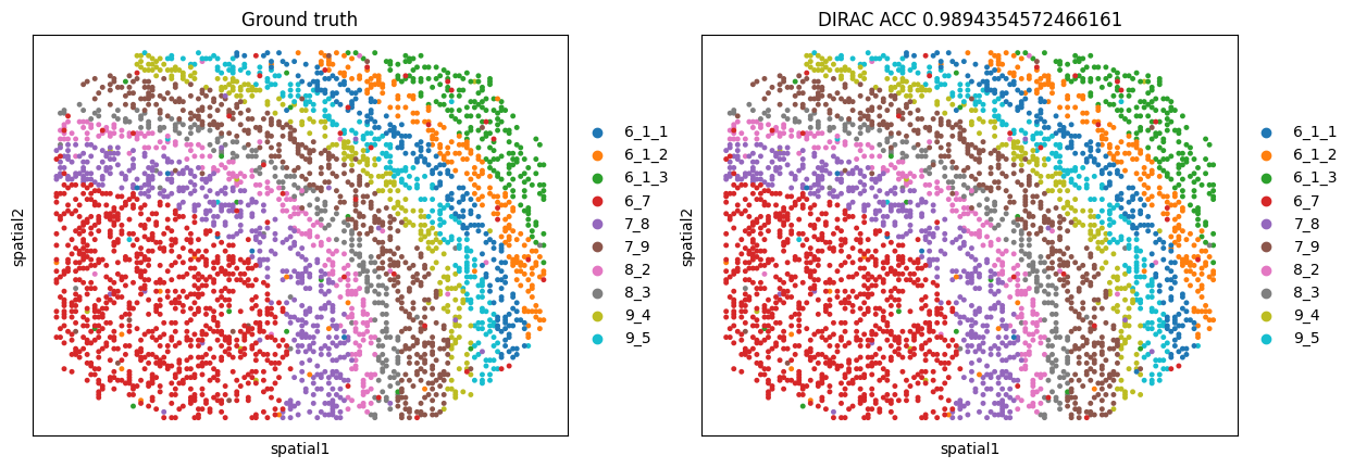
6. Dual-Modality Annotation (RNA+ATAC → RNA+ATAC)¶

What this part does

Concatenates RNA and ATAC features per cell and performs label transfer across modalities.
Uses combine_multimodal_adatas(...) to build a single AnnData with stacked features.
Provides a split_list to tell DIRAC where each modality lives in the concatenated matrix.

Subgraph-settings(num_part)

The spatial graph is split into num_parts_* subgraphs. More parts → smaller subgraphs → lower peak memory but more overhead.
Ensure at least 1 part: max(1, n_cells // 200).
When to increase: GPU OOM or very large tissues.

Notes on ``split_list``

It must enumerate non-overlapping half-open ranges (start, end) that exactly cover the concatenated feature columns.
Make sure the ranges line up with the same order you used in combine_multimodal_adatas({...}).

Step-by-step

[4]:

# 1) Load inputs
# RNA
source_adata_RNA = anndata.read_h5ad(os.path.join(data_path, "source_RNA.h5ad"))
target_adata_RNA = anndata.read_h5ad(os.path.join(data_path, "target_RNA.h5ad"))
print(source_adata_RNA); print(target_adata_RNA)

# ATAC
source_adata_ATAC = anndata.read_h5ad(os.path.join(data_path, "source_ATAC.h5ad"))
target_adata_ATAC = anndata.read_h5ad(os.path.join(data_path, "target_ATAC.h5ad"))
print(source_adata_ATAC); print(target_adata_ATAC)

# 2) Preprocess each modality
sc.pp.normalize_total(source_adata_RNA);  sc.pp.log1p(source_adata_RNA);  sc.pp.scale(source_adata_RNA)
sc.pp.normalize_total(target_adata_RNA);  sc.pp.log1p(target_adata_RNA);  sc.pp.scale(target_adata_RNA)

sc.pp.normalize_total(source_adata_ATAC); sc.pp.log1p(source_adata_ATAC); sc.pp.scale(source_adata_ATAC)
sc.pp.normalize_total(target_adata_ATAC); sc.pp.log1p(target_adata_ATAC); sc.pp.scale(target_adata_ATAC)

# 3) Concatenate modalities (feature-wise)
source_adata = sd.utils.combine_multimodal_adatas({"RNA": source_adata_RNA, "ATAC": source_adata_ATAC})
target_adata = sd.utils.combine_multimodal_adatas({"RNA": target_adata_RNA, "ATAC": target_adata_ATAC})

# 4) Spatial graphs
source_edge_index = sd.utils.get_multi_edge_index(source_adata.obsm["spatial"], source_adata.obs["batch"], n_neighbors=10)
target_edge_index = sd.utils.get_single_edge_index(target_adata.obsm["spatial"], n_neighbors=10)

# 5) Initialize DIRAC annotation app
annotate = sd.main.annotate_app(save_path=save_path, use_gpu=True)

# 6) Define modality splits in the concatenated matrix
#  RNA: [0, dim_RNA)
#  ATAC: [dim_RNA, dim_RNA + dim_ATAC)
split_list = [
        (0, source_adata_RNA.shape[1]),
        (source_adata_RNA.shape[1], source_adata_RNA.shape[1] + source_adata_ATAC.shape[1]),
    ]

# 7) Package data (note split_list)
samples = annotate._get_data(
        source_data=source_adata.X,
        source_label=source_adata.obs["cell.type"],
        source_edge_index=source_edge_index,
        target_data=target_adata.X,
        target_edge_index=target_edge_index,
        num_parts_source=source_adata.shape[0] // 200,
        num_parts_target=target_adata.shape[0] // 200,
        split_list=split_list,
    )

# 8) Build model and train
models = annotate._get_model(samples=samples, opt_GNN="SAGE")
results = annotate._train_dirac_annotate(samples=samples, models=models, n_epochs=100)

# 9) Write back outputs
source_adata.obsm[f"{methods}_embed"] = results["source_feat"]
target_adata.obsm[f"{methods}_embed"] = results["target_feat"]
target_adata.obs[f"{methods}_pred"] = results["target_pred"]
target_adata.obs[f"{methods}"] = target_adata.obs[f"{methods}_pred"].map(results["pairs"])

# 10) Metrics & Visualization
metrics_all = {
            "Accuracy Score":
                float(sklearn.metrics.accuracy_score(target_adata.obs["cell.type"], target_adata.obs[f"{methods}"])),
            "Precision Score":
                float(sklearn.metrics.precision_score(target_adata.obs["cell.type"], target_adata.obs[f"{methods}"], average='weighted')),
            "Recall Score":
                float(sklearn.metrics.recall_score(target_adata.obs["cell.type"], target_adata.obs[f"{methods}"], average='weighted')),
            "F1 Score":
                float(sklearn.metrics.f1_score(target_adata.obs["cell.type"], target_adata.obs[f"{methods}"], average='weighted'))}
print(metrics_all)

sc.pl.embedding(target_adata, basis='spatial', color=['cell.type', f'{methods}'], title=['Ground truth',f"{methods} ACC {metrics_all['Accuracy Score']}"], s=50, show=False)

AnnData object with n_obs × n_vars = 11971 × 200
    obs: 'pop', 'depth', 'cell.type', 'cell.type.idx', 'batch'
    obsm: 'spatial'
AnnData object with n_obs × n_vars = 3029 × 200
    obs: 'pop', 'depth', 'cell.type', 'cell.type.idx', 'batch'
    obsm: 'spatial'
AnnData object with n_obs × n_vars = 11971 × 600
    obs: 'pop', 'depth', 'cell.type', 'cell.type.idx', 'batch'
    obsm: 'spatial'
AnnData object with n_obs × n_vars = 3029 × 600
    obs: 'pop', 'depth', 'cell.type', 'cell.type.idx', 'batch'
    obsm: 'spatial'
Average neighbors per node (directed): 10.00 (edges=119710, nodes=11971)
Average neighbors per node (directed): 10.00 (edges=30290, nodes=3029)
Identified 2 unique domains.

Computing METIS partitioning...
Done!
Computing METIS partitioning...
Done!
DIRAC annotate training..: 100%|█| 10

{'Accuracy Score': 0.9894354572466161, 'Precision Score': 0.9894781692014127, 'Recall Score': 0.9894354572466161, 'F1 Score': 0.9894421771682003}

[4]:

[<Axes: title={'center': 'Ground truth'}, xlabel='spatial1', ylabel='spatial2'>,
 <Axes: title={'center': 'DIRAC ACC 0.9894354572466161'}, xlabel='spatial1', ylabel='spatial2'>]

../_images/notebooks_run-scMultiSim_11_4.png

7. Novel Cell Type Discovery (Confidence Filtering)¶

Why this matters. Real references are often incomplete: some cell types may be absent. Here we intentionally drop two cell types from the reference, train DIRAC, and then use a confidence threshold (default 0.9, tunable) to mark low-confidence predictions as ``”unassigned”``. This flags putative novel/unknown or out-of-reference cell types in the target.

What happens.

Randomly remove two reference cell types ('7_9', '6_1_2' in this demo).
Train DIRAC on the pruned reference and full target (RNA+ATAC).
Use filter_low_confidence=True with confidence_threshold=0.9.
Post-process: points below the threshold become "unassigned".
Report metrics on the remaining assigned cells and visualize confidence.

Tip. Increase the threshold (e.g., 0.95) for stricter assignment; relax it (e.g., 0.8) on noisier data.

[5]:

 # 1) Load inputs
# RNA
source_adata_RNA = anndata.read_h5ad(os.path.join(data_path, "source_RNA.h5ad"))
target_adata_RNA = anndata.read_h5ad(os.path.join(data_path, "target_RNA.h5ad"))
print(source_adata_RNA); print(target_adata_RNA)

# ATAC
source_adata_ATAC = anndata.read_h5ad(os.path.join(data_path, "source_ATAC.h5ad"))
target_adata_ATAC = anndata.read_h5ad(os.path.join(data_path, "target_ATAC.h5ad"))
print(source_adata_ATAC); print(target_adata_ATAC)

####### remove some cell types from reference data
drop_celltypes = ['7_9', '6_1_2']
source_adata_RNA = source_adata_RNA[~source_adata_RNA.obs['cell.type'].isin(drop_celltypes)].copy()
source_adata_ATAC = source_adata_ATAC[~source_adata_ATAC.obs['cell.type'].isin(drop_celltypes)].copy()

# 2) Preprocess each modality
sc.pp.normalize_total(source_adata_RNA);  sc.pp.log1p(source_adata_RNA);  sc.pp.scale(source_adata_RNA)
sc.pp.normalize_total(target_adata_RNA);  sc.pp.log1p(target_adata_RNA);  sc.pp.scale(target_adata_RNA)

sc.pp.normalize_total(source_adata_ATAC); sc.pp.log1p(source_adata_ATAC); sc.pp.scale(source_adata_ATAC)
sc.pp.normalize_total(target_adata_ATAC); sc.pp.log1p(target_adata_ATAC); sc.pp.scale(target_adata_ATAC)

# 3) Concatenate modalities (feature-wise)
source_adata = sd.utils.combine_multimodal_adatas({"RNA": source_adata_RNA, "ATAC": source_adata_ATAC})
target_adata = sd.utils.combine_multimodal_adatas({"RNA": target_adata_RNA, "ATAC": target_adata_ATAC})

# 4) Spatial graphs
source_edge_index = sd.utils.get_multi_edge_index(source_adata.obsm["spatial"], source_adata.obs["batch"], n_neighbors=10)
target_edge_index = sd.utils.get_single_edge_index(target_adata.obsm["spatial"], n_neighbors=10)

# 5) Initialize DIRAC annotation app
annotate = sd.main.annotate_app(save_path=save_path, use_gpu=True)

# 6) Define modality splits in the concatenated matrix
#  RNA: [0, dim_RNA)
#  ATAC: [dim_RNA, dim_RNA + dim_ATAC)
split_list = [
        (0, source_adata_RNA.shape[1]),
        (source_adata_RNA.shape[1], source_adata_RNA.shape[1] + source_adata_ATAC.shape[1]),
    ]

# 7) Package data (note split_list)
samples = annotate._get_data(
        source_data=source_adata.X,
        source_label=source_adata.obs["cell.type"],
        source_edge_index=source_edge_index,
        target_data=target_adata.X,
        target_edge_index=target_edge_index,
        num_parts_source=source_adata.shape[0] // 200,
        num_parts_target=target_adata.shape[0] // 200,
        split_list=split_list,
    )

# 8) Build model and train
models = annotate._get_model(samples=samples, opt_GNN="SAGE")
results = annotate._train_dirac_annotate(samples=samples, models=models, n_epochs=100,
                                         filter_low_confidence = True, # enable filtering
                                         confidence_threshold = 0.9) # tune this (e.g., 0.8–0.95)

# 9) Write back outputs
target_adata.obs[f"{methods}_pred"] = results["target_pred_filtered"]
target_adata.obs[f"{methods}"] = target_adata.obs[f"{methods}_pred"].map(results['pairs_filter'])
target_adata.obs["Confidence"] = results['target_confs']

# 10) Metrics (on assigned cells only) & Visualization
valid_mask = target_adata.obs[f"{methods}"] != "unassigned"
filtered_target = target_adata[valid_mask].copy()
metrics_all = {
                "Accuracy Score": float(sklearn.metrics.accuracy_score(
                    filtered_target.obs["cell.type"],
                    filtered_target.obs[f"{methods}"])),
                "Precision Score": float(sklearn.metrics.precision_score(
                    filtered_target.obs["cell.type"],
                    filtered_target.obs[f"{methods}"],
                    average='weighted', zero_division=0)),
                "Recall Score": float(sklearn.metrics.recall_score(
                    filtered_target.obs["cell.type"],
                    filtered_target.obs[f"{methods}"],
                    average='weighted')),
                "F1 Score": float(sklearn.metrics.f1_score(
                    filtered_target.obs["cell.type"],
                    filtered_target.obs[f"{methods}"],
                    average='weighted')),
                "Unassigned Rate": float(1 - len(filtered_target)/len(target_adata))
                    }
sc.pl.embedding(target_adata, basis='spatial', color=['cell.type', f'{methods}', "Confidence"],
                title=['Ground truth',f"DIRAC ACC {metrics_all['Accuracy Score']}", "Confidence"],
                s=80, show=False, color_map="CMRmap")

AnnData object with n_obs × n_vars = 11971 × 200
    obs: 'pop', 'depth', 'cell.type', 'cell.type.idx', 'batch'
    obsm: 'spatial'
AnnData object with n_obs × n_vars = 3029 × 200
    obs: 'pop', 'depth', 'cell.type', 'cell.type.idx', 'batch'
    obsm: 'spatial'
AnnData object with n_obs × n_vars = 11971 × 600
    obs: 'pop', 'depth', 'cell.type', 'cell.type.idx', 'batch'
    obsm: 'spatial'
AnnData object with n_obs × n_vars = 3029 × 600
    obs: 'pop', 'depth', 'cell.type', 'cell.type.idx', 'batch'
    obsm: 'spatial'

Computing METIS partitioning...
Done!
Computing METIS partitioning...
Done!

Average neighbors per node (directed): 10.00 (edges=95610, nodes=9561)
Average neighbors per node (directed): 10.00 (edges=30290, nodes=3029)
Identified 2 unique domains.

DIRAC annotate training..: 100%|█| 10

[5]:

[<Axes: title={'center': 'Ground truth'}, xlabel='spatial1', ylabel='spatial2'>,
 <Axes: title={'center': 'DIRAC ACC 0.9123914759273876'}, xlabel='spatial1', ylabel='spatial2'>,
 <Axes: title={'center': 'Confidence'}, xlabel='spatial1', ylabel='spatial2'>]

../_images/notebooks_run-scMultiSim_13_5.png

Summary

Single-modality (RNA→RNA): build source/target spatial graphs → train with GraphSAGE → predict → metrics → spatial maps.
Dual-modality (RNA+ATAC): concatenate features and provide split_list; rest is identical.
Novel cell type discovery: train with confidence filtering to mark “unassigned” cells when the reference is incomplete; report Unassigned Rate alongside standard metrics.
Use num_parts_* to trade memory for speed, and tune neighbors/model/thresholds for stable, well-mixed embeddings and reliable annotations.